Predicting international house prices
What factors influence house prices? This is a perennial topic of dinner party discussion, but the standard of the debate rarely rises above offering anecdotal evidence. Frustrated with the status quo, I decided to tackle the question with statistics. In this post I look at which macroeconomic factors are associated with future house price rises or falls.
(This post is not intended to be investment advice and does not represent the opinions of my employer.)
To do this, I perform a Fama-MacBeth regression:
- I gathered quarterly timeseries for several macro factors covering many countries, plus quarterly house price returns in those countries
- For each quarter in my sample, I perform a linear regression to predict next quarter’s house price returns from this quarter’s macro factors.
- Now I have, for each factor, a timeseries of regression coefficients. If a hypothesis test rejects the null that this timeseries has zero mean, there is a statistically significant association between the factor and future returns.
I tested several factors that have channels of potential causality to house prices:
- Rent: if houses yield a lot of rent relative to their price, they could rise in price as people do e.g. more buy-to-let transactions
- Affordability: house prices that are low relative to income could imply that housing will rise in the future
- Past price rises: if house prices have risen in the recent past, this might continue in the future
- Population growth: if the population is growing you might expect prices to rise as supply struggles to keep up
- Economic growth measured several ways (GDP growth, median wage growth, per-capita consumption growth etc): if people have more money to spend they might use some of it to bid up existing houses
- Interest rates: low rates make it easier to take out a big mortgage which lets them spend more on housing
- National indebtedness: if people already carry a lot of debt they might be unwilling to take on a lot of housing debt, which could help hold valuations down
In brief: my findings are that house prices rise most quickly in countries where prices have risen in the past one year, which offer attractive rental yields, have experienced high per-capita consumption growth over the last year, and have low short-term interest rates. The other factors tested are either subsumed by one of these strong predictors, or seem unrelated (at least, as far as I can tell given my sample: weak effects might only be discoverable in the presence of data from more countries and time periods).
My methodology is similar to that of Case and Shiller in their 1990 paper “Forecasting Prices and Excess Returns in the Housing Market”. The key difference are that I consider the international housing market, while they look at the difference between US states, and they only look at a subset of the variables that I consider. I also have the advantage of having 30 years more data than they do!
The countries in my sample were as follows:
- Developed Europe: Austria (AUT), Belgium (BEL), Switzerland (CHE), Germany (DEU), Denmark (DNK), Spain (ESP), Finland (FIN), France (FRA), the United Kingdom (GBR), Ireland (IRL), Iceland (ISL), Italy (ITA), Luxembourg (LUX), the Netherlands (NLD), Norway (NOR), Portugal (PRT), Sweden (SWE)
- Emerging Europe: Czechia (CZE), Estonia (EST), Greece (GRC), Hungary (HUN), Lithuania (LTU), Latvia (LVA), Poland (POL), Russia (RUS), Slovakia (SVK), Slovenia (SVN)
- Asia: Australia (AUS), China (CHN), Indonesia (IDN), India (IND), Israel (ISR), Japan (JPN), Korean (KOR), New Zealand (NZL)
- North America: Canada (CAN), Mexico (MEX), the USA (USA)
- South America: Chile (CHL), Colombia (COL)
- Africa: South Africa (ZAF)
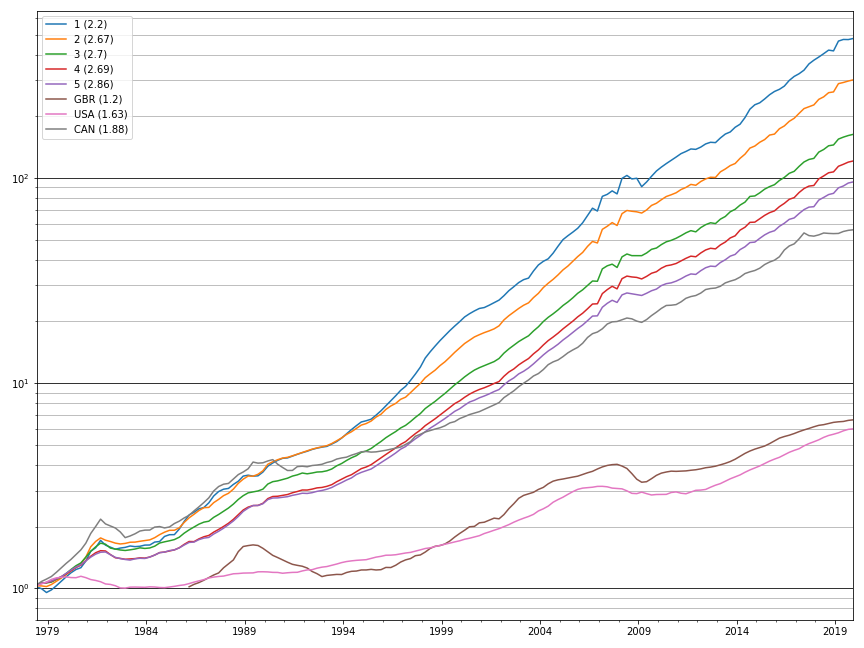
If you had borrowed money at the prevailing local-currency short-term interest rate and invested it in housing in the top 3 countries in this list as picked by my model 1, you would have grown your initial borrowing almost 900% from 1979 to 2020. This far outpaces the approximately 40% cumulative growth that you would have experienced in, say, the USA or Canada during that time:
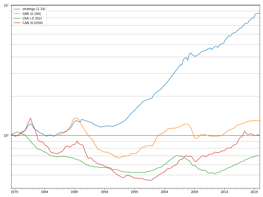
If UK/USA/Canadian house price appreciation looks a bit lower than you are expecting in this graph, remember that interest costs have been deducted from all the timeseries here, and I don’t include any income you would have made from renting the property out.
This graph makes it look like you’d be crazy not to following my trading strategy rather than own a home in a single country for a long period of time. However, the graph is misleading in that I have made no provision for transaction costs – in reality you’d end up giving a lot of the strategy return back in the shape of real estate agent fees and housing transaction tax (“stamp duty” in the UK).
As one estimate of tranasction costs, consider that UK stamp duty is roughly 2%, real estate agent fees are about 1.5% and you could reasonably incur many other costs (e.g. conveyancing and mortgage arrangement fees) adding up to 0.5% for a total 4% cost every time you switch the house you own. If you switched houses every quarter over the 168 quarters from 1979 to 2020, that would imply that 672% of your 900% return would be eaten by fees! In reality you would want to switch houses less frequently than this, but it would still be a drag on strategy returns.
In the following sections I dive further into the technical detail of the model and discuss other trading strategies that you might use to exploit this model.
Which returns?
How do you measure the returns to housing investment? One naive method is to look at the average selling price within each period, and say that the extent to which this grows from period to period represents the returns which a homeowner would have experienced. However, this is obviously flawed:
- The houses being sold at time T are different to those that we were sold at time T-1, so you are not measuring the price change in a fixed housing investment.
- People are unwilling to sell houses if they would realize a loss, so the housing transactions countributing to the average are mostly drawn from the sample of homes with higher-than-average appreciation.
- This methodology does not take account of quality improvements that have been made to houses between sales (e.g. regular maintenance, refurbishment or extension).
These factors tend to bias up the reported returns to housing investment. Economists are well aware of these issues and have a few measurement methods that try to adjust for the bias. I principally rely on house price returns from the Dallas Fed’s house price indexes, which use the repeat-sales method to help debias. In this method, returns are estimated by looking at the average price growth experienced at any given fixed addresses, which avoids e.g. the returns being biased upwards if most housing transactions are of expensive new-builds. For countries not covered by the Dallas Fed, I estimate returns using OECD’s average-sale-price index.
I do not attempt to subtract maintenance or improvement costs from returns, which is definitely a flaw in my methodology. Unfortunately I don’t have good data about how these costs vary between countries so it’s not clear how to do better here.
I measure all returns in local currency terms, subtracting the local short-term interest rate, to give which are usually called “excess returns”. This is the metric we should use if we imagine that we are foreign investors in the local property market and we hedge our foreign exchange risk by selling a FX swap so that we don’t lose or gain money if exchange rates moves.
For example, imagine that we are a UK based investor in Turkish property. If Turkish property appreciates 20% but the Turkish Lira falls 14% against the pound we’ve only made a 6% gain. On the face of it, we’ll be taking on a lot of foreign exchange risk: the Lira is volatile, and we could easily lose 40% of our investment in a year just due to Lira depreciation. The smart thing to do is to enter into a GBP/TRY swap in the amount of our real estate investment: if TRY depreciates, we will gain money on the swap that offsets our real estate losses, i.e we are hedged with respect to currency movements.
The cost of a FX swap like this depend on the interest rate differential between the two countries: if GBP interest rates are 1% and Turkish rates are 12% then we’ll have to pay 11% annually to sell TRY via this swap, so our expected return on the Turkish real estate investment is equal to the expected return in local currency returns minus Turkish rates, plus GBP rates. Because GBP rates are the same regardless of which country we are investing in, in order to compare countries in which we might invest, we are most interested in predicting local currency returns minus local rates i.e. excess returns.
Other options would be to predict:
- Returns in local currency terms without adjustment for short-term interest rates: this is flawed because it overstates the returns available from investing in countries with very high inflation
- Returns in dollar terms: this is the best variable to predict if you are going to make real estate investments in foreign countries without hedging the FX risk. However, the dollar FX rate introduces considerable noise into the returns which greatly weakens the power of our statistical tests.
- Real returns in local currency terms. This avoids overstating the returns available in high-inflation countries, and does not introduce USD FX rate noise, but it’s not possible to guarantee that you will actually earn real returns, so the practical relevance of predicting these returns is unclear. Although there is clearly a positive association between high interest rates and high inflation, FX swaps cost an amount proportional to the interest rate and not proportional to the inflation rate.
I do not include rental income in the returns that I’m trying to predict because there is usually little uncertainty about the yield you will earn, so there is no need to model it!
Population growth
I obtained population data from the OECD and performed a Fama-MacBeth regression predicting excess returns from some of the fields.
This table summarizes the results: each column represents one model, the cells holding the average regression coefficient, the t-statistic for the regression coefficient timeseries, and a number of stars summarizing the p-value 2 from * (p < 0.05) to ** (p < 0.01) or *** (p < 0.005).
| 0 | 1 | 2 | |
|---|---|---|---|
| population_15_to_64_growth | 0.00928 (0.026) | 2.48 (2.61) | |
| population_15_to_64_fraction | -0.00364 (-0.09) | 0.00552 (0.145) | -0.0248 (-0.582) |
| population_total_growth | -0.232 (-0.515) | -3.41* (-2.94) |
The only population model which shows a significant coefficient is one which includes both the growth rate in the total population and the 15-64 growth rate, and the coefficient on the two rates have opposite signs. This looks like a clearly spurious result caused by the colinearity of these two variables.
Interestingly, if you include rental income in the returns then there is a weak positive association with population growth. So (weirdly) it appears that population growth causes high rental yields, but not house price appreciation:
| 0 | 1 | 2 | |
|---|---|---|---|
| population_15_to_64_growth | 1.79** (4.67) | 8.43* (4.23) | |
| population_15_to_64_fraction | -0.0232 (-0.525) | 0.0256 (0.568) | -0.194* (-3.17) |
| population_total_growth | 2.25* (3.89) | -10.4 (-2.89) |
Economic growth
I take quarterly median wage growth from the OECD wage database, and real GDP and private consumption growth from the OECD quarterly national accounts data. I tested both quarterly data, and rolling means evaluated over the trailing year of data (to smooth out intra-year variation). Regression results are as follows:
| 0 | 1 | 2 | 3 | 4 | 5 | 6 | 7 | 8 | 9 | |
|---|---|---|---|---|---|---|---|---|---|---|
| real_wage_growth | 0.508*** (4.06) | 0.0768 (0.705) | ||||||||
| local_real_personal_disposable_income_growth | 0.227*** (3.62) | 0.154* (2.47) | ||||||||
| real_private_consumption_growth | 0.396*** (6.7) | 0.26*** (3.89) | ||||||||
| real_gdp_growth | 0.314*** (5.76) | 0.0945 (1.56) | ||||||||
| real_wage_growth_1y | 0.116* (3.3) | -0.0372 (-1.15) | ||||||||
| local_real_personal_disposable_income_growth_1y | 0.161*** (7.38) | 0.0221 (0.79) | ||||||||
| real_private_consumption_growth_1y | 0.153*** (9.14) | 0.0967*** (3.79) | ||||||||
| real_gdp_growth_1y | 0.151*** (6.56) | 0.0559 (2.27) |
Broadly, the pattern is that real per-capita private consumption growth has the strongest association with future house price appreciation, and the magnitude of this is quite large: a 1% increase in consumption predicts a 0.15% to 0.4% increase in house prices.
Momentum
In most markets, recent price changes tend to continue into the future. This is an one of the most robust observations in quantitative finance, and it has been validated as being true from as early as 1880. It seems that housing is no exception to this rule: the average rate of price growth over the last year is a strong prediction of future returns:
| 0 | 1 | 2 | 3 | |
|---|---|---|---|---|
| momentum | 0.174*** (14.9) | -0.0195 (-0.592) | ||
| excess_momentum | 0.177*** (18.2) | 0.227*** (6.86) | ||
| usd_momentum | 0.0911*** (12) | -0.0317 (-1.72) |
Here I have tested the rate of growth as computed from local returns (momentum), from excess returns, and from dollar returns. Each works, but the strongest prediction of future excess returns is the measure calculated from excess returns themselves. The model suggests that if prior period returns were 1%, then next period returns are expected to be be 0.18%.
This is a fairly short-term effect. If you lag the momentum variable by 1 year it has no predictive power, and looking at the momentum effect from the prior 6 quarters separately (rather than taking the mean of the first 4 to form excess_momentum) we find that only the first 4 quarters get a significant positive coefficient:
| 0 | 1 | |
|---|---|---|
| excess_momentum | 0.198*** (17.5) | |
| excess_momentum_lag_1y | -0.0165 (-1.79) | |
| excess_momentum_lag0 | 0.385*** (8.25) | |
| excess_momentum_lag1 | 0.197** (2.54) | |
| excess_momentum_lag2 | 0.106* (1.87) | |
| excess_momentum_lag3 | 0.179*** (3.75) | |
| excess_momentum_lag4 | -0.113* (-1.74) | |
| excess_momentum_lag5 | -0.0071 (-0.116) |
Value and carry
Momentum is the most famous quantitative factor, but “value” and “carry” are almost as famous. Value is the idea that assets that have a low market price relative to their “fundamental” value will tend to outperform in the future, and “carry” is roughly the idea that assets that are expected to yield a lot of cashflow relative to their market price will outperform.
In housing investment, the obvious “value” measure is to look at the ratio of incomes to house prices. If a country has incomes that are low relative to house prices, that housing market might be overvalued. “Carry” is simply the rental yield, and if housing is like other markets we expect countries with high rental yields to have house prices that appreciate in the future.
Rental yield and price-to-income are available in the OECD housing database, but only as indexes which are normalized such that all countries have value 100 in the index as of 2015. This frustrates cross-country comparison, so I convert from the index to an absolute level of rental yield and price-to-income by scaling the index such that the last observation matches the rental yield/price-to-income data from Global Property Guide and Numbeo, two great resources for quantitative data about the current state of the housing market worldwide.
Regressing the value and carry factors together with momentum, we do see roughly the expected pattern, but it is very weak compared to momentum:
| 0 | 1 | 2 | 3 | |
|---|---|---|---|---|
| momentum | 0.177*** (7.68) | |||
| carry | -0.0113 (-0.138) | 0.1 (1.15) | 0.0609 (0.602) | 0.159 (1.53) |
| value | 0.00375** (3.63) | 0.00189 (1.56) | 0.00416** (3.35) | 0.00276 (2.24) |
| excess_momentum | 0.174*** (13) | |||
| usd_momentum | 0.0834*** (6.01) |
The “value” effect is not always statistically significant, but the coefficient always has the right sign. The “carry” effect is never significant but has the right sign in the most important specification, where momentum is measured via excess_momentum.
Interest rates
I take long and short term interest rates from the OECD MEI database. I form the “ranked” version of each of these by sorting countries on the interest rate variable and then assigning countries a real number in the range -1 to 1 which is a linear function of their index after sorting. Interest rates exhibit very strong dispersion across countries, and ranking helps avoid the regression results being driven purely by one or two outlier countries.
| 0 | 1 | 2 | 3 | 4 | |
|---|---|---|---|---|---|
| short_term_rates | -0.93*** (-5.65) | -0.593*** (-6.36) | |||
| long_term_rates | 0.397 (1.84) | -0.625*** (-5.05) | |||
| rank_short_term_rates | -0.00836*** (-5.87) | ||||
| rank_long_term_rates | 0.00114 (0.811) | -0.00595*** (-6.78) |
As you would expect, high short term rates are associated with lower excess returns in the future: a 1% higher short term rate means 0.6% lower price appreciation. This is partly a mechanical effect, since excess returns are defined as local price returns minus short term rates, but in fact this pattern remains even if we predcit local price returns instead:
| 0 | 1 | 2 | 3 | 4 | |
|---|---|---|---|---|---|
| short_term_rates | -0.404 (-2.67) | -0.326*** (-3.55) | |||
| long_term_rates | 0.155 (0.821) | -0.527* (-2.32) | |||
| rank_short_term_rates | -0.00284 (-2.04) | ||||
| rank_long_term_rates | -0.000378 (-0.284) | -0.00316*** (-3.44) |
Household indebtedness
In this set of tests, I take indebtedness measures from the OECD annual national accounts data. I don’t find an association between any of these features and future returns:
| 0 | 1 | 2 | 3 | 4 | 5 | 6 | 7 | |
|---|---|---|---|---|---|---|---|---|
| household_saving_fraction | 0.022 (0.792) | -0.000814 (-0.0259) | ||||||
| household_debt_fraction | 0.000586 (0.463) | 0.000552 (0.428) | ||||||
| net_lending_pct_gdp | -0.0368 (-1.3) | 0.00645 (0.188) | ||||||
| rank_household_saving_fraction | -0.000316 (-0.139) | -0.000481 (-0.455) | ||||||
| rank_household_debt_fraction | 4.15e-05 (0.0258) | -3.97e-05 (-0.0254) | ||||||
| rank_net_lending_pct_gdp | -0.000689 (-0.419) | -0.00077 (-0.839) |
Rental growth
I take measures of rental growth as used to compute OECD consumer price indexes and regress returns on them. If anything it seems like rental growth is negative related to future price returns, which is the opposite of what I would expect. The relationship is weak, however, with only one model showing a weak significant result:
| 0 | 1 | 2 | 3 | 4 | 5 | |
|---|---|---|---|---|---|---|
| cpi_actual_rentals | -0.239* (-1.46) | |||||
| cpi_actual_rentals_1y | -0.039 (-1.31) | |||||
| rank_cpi_actual_rentals_1y | -0.00182 (-1.16) | |||||
| cpi_imputed_rentals | 1.15 (1.26) | |||||
| cpi_imputed_rentals_1y | 0.00429 (0.107) | |||||
| rank_cpi_imputed_rentals_1y | -0.000391 (-0.3) |
Composite model
Taking the most robust predictors from each of the models above, we can form a model that simultaneously takes account of all these factors:
| 0 | |
|---|---|
| excess_momentum | 0.146*** (14.4) |
| carry | 0.314*** (3.74) |
| value | 0.000202 (0.199) |
| real_private_consumption_growth_1y | 0.0858*** (3) |
| short_term_rates | -0.496*** (-6.43) |
This model has an average R-squared of 58%, meaning it explains almost two thirds of the variation in the international cross-section of house price returns.
If we try to predict returns inclusive of rental income, the carry factor obviously becomes much more important but the others remain mostly unaffected:
| 0 | |
|---|---|
| excess_momentum | 0.14*** (13.9) |
| carry | 1.29*** (15.6) |
| value | 0.00028 (0.279) |
| real_private_consumption_growth_1y | 0.0843*** (3.02) |
| short_term_rates | -0.5*** (-6.59) |
Which countries are the best investments as of the time of writing this post? From best (rank 0) to worst (rank 33):
| ex rental yield | inc rental yield | |
|---|---|---|
| 0 | LVA | LVA |
| 1 | PRT | PRT |
| 2 | SVK | SVK |
| 3 | HUN | HUN |
| 4 | SVN | SVN |
| 5 | GRC | LTU |
| 6 | LTU | GRC |
| 7 | EST | POL |
| 8 | POL | IRL |
| 9 | LUX | EST |
| 10 | AUT | LUX |
| 11 | NLD | NLD |
| 12 | CZE | BEL |
| 13 | BEL | AUT |
| 14 | IRL | DNK |
| 15 | DNK | CZE |
| 16 | DEU | ESP |
| 17 | SWE | USA |
| 18 | ESP | DEU |
| 19 | FRA | SWE |
| 20 | FIN | FIN |
| 21 | USA | ITA |
| 22 | NOR | NOR |
| 23 | CHE | CHL |
| 24 | ITA | FRA |
| 25 | CHL | CHE |
| 26 | JPN | CAN |
| 27 | GBR | NZL |
| 28 | NZL | GBR |
| 29 | CAN | JPN |
| 30 | KOR | ZAF |
| 31 | AUS | AUS |
| 32 | ZAF | RUS |
| 33 | RUS | KOR |
Trading strategy
If we could short housing, one way to exploit this model would be to go long or short housing in proportion to the expected returns estimate from our best model as of n periods ago. If we did this, our returns would look like this, where n ranges from 0 to 8:
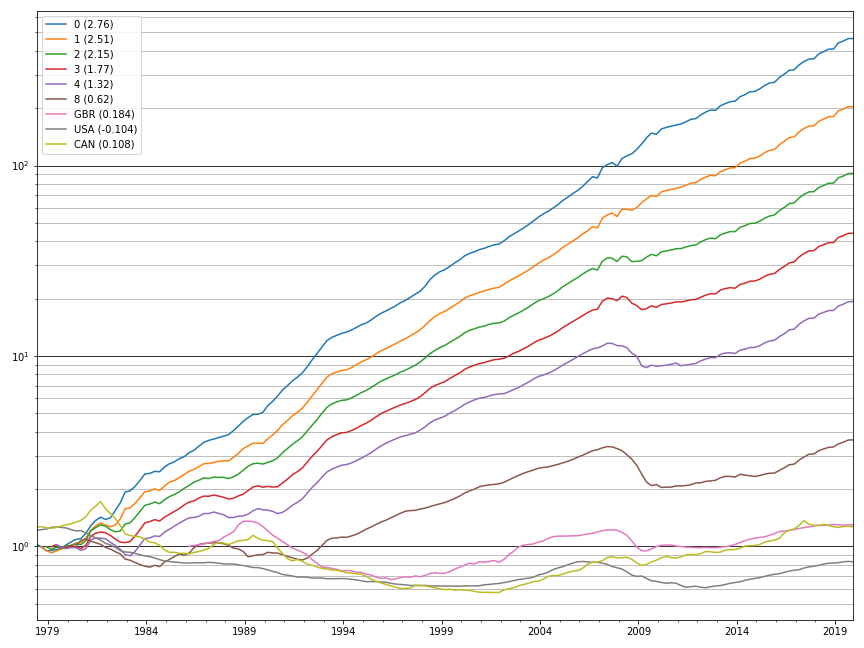
The number in brackets in the legend of this chart is the Sharpe ratio i.e. the ratio of the mean return of the strategy within a year to the standard deviation of the strategy within that year. The Sharpe Ratio is the best measure of how good a trading strategy is, and our best result here of 2.76 is very respectable: as a point of comparison, the US stock market has been doing extremely well over the last few years, and it has realized a Sharpe of only 1 or so.
Unfortunately, we can’t short the housing market, so a more realistic strategy is hold all countries in proportion to their expected return, but avoid holding any with expected negative returns:
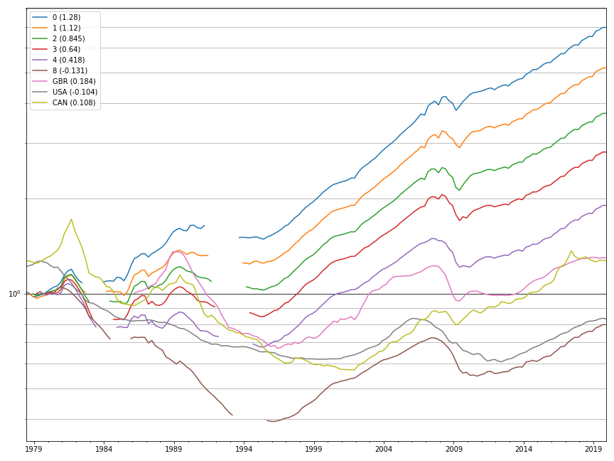
(Note that from 1991 to 1994 this strategy is entirely invested in cash because all countries are expected to underperform.)
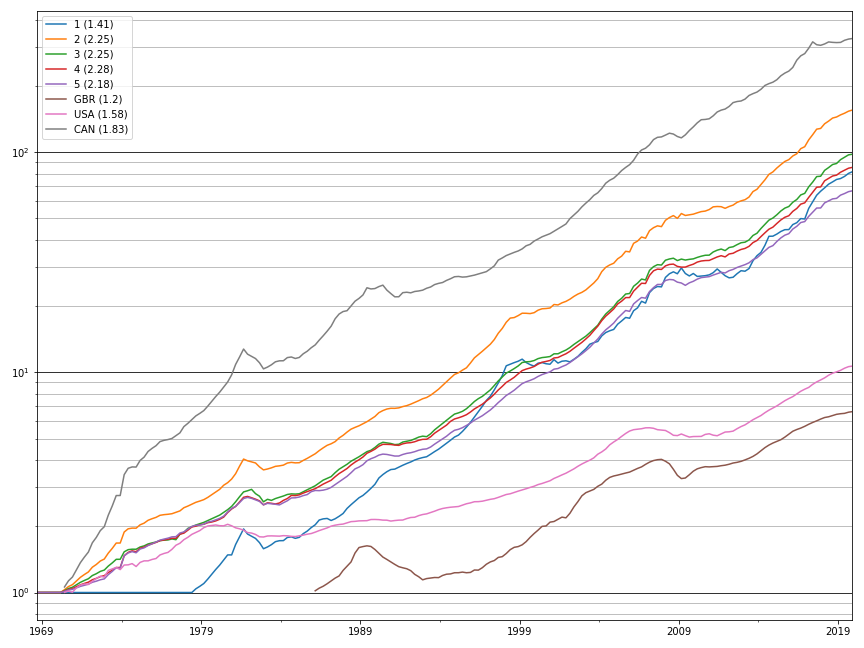
Another idea is to hold just the top n countries, where n ranges from 1 to 5:
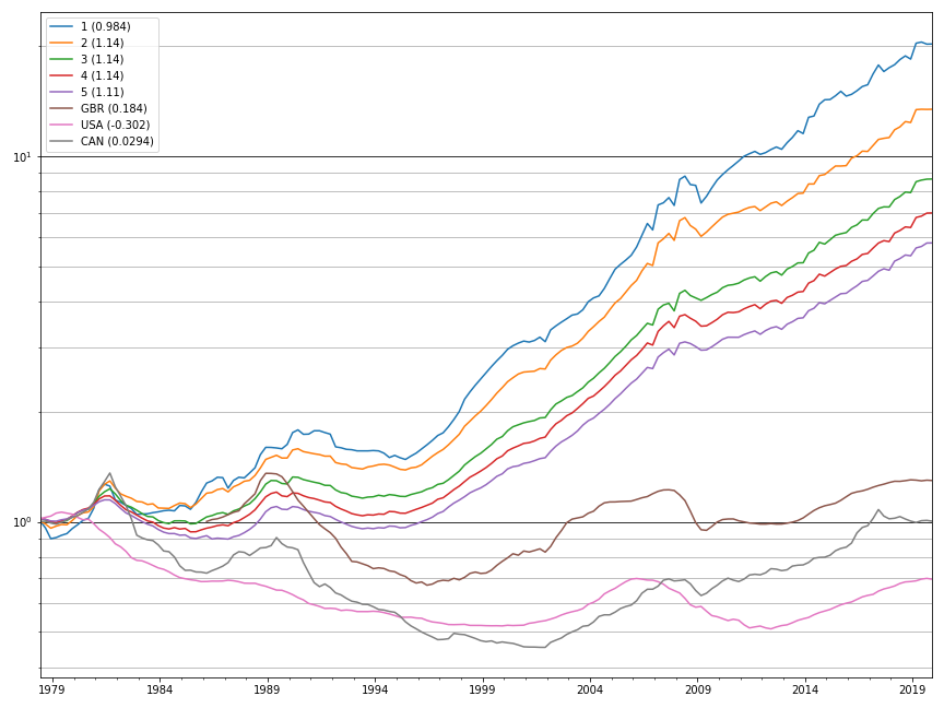
Note that all of these strategies completely ignore the rental income portion of the return. This makes a big difference. If we set the expected rental return in the next period equal to the return over the previous period and then buy housing in the top n countries according to this metric, then our total return (including rental income) is much more strongly positive, with a maximum Sharpe of 2.86:
Strikingly, you can get results almost as good by just purchasing housing in the countries exhibiting the highest current rental yield, which is a strategy commonly employed by housing speculators in the UK:
Conclusion
House prices are strongly predictable (R-squared 58%) and mostly driven by momentum, rental yields, per-capita consumption growth, and short term interest rates. Trading strategies based on buying just those countries with the highest predicted price appreciation appear to realize very high, economically significant, Sharpe ratios, but it’s unclear how implementable these are given high transaction costs and the long-only nature of the housing market. The impact of government housing ownership regulations and taxes is also uncertain but this would certainly drag down returns somewhat. The dubious nature of house price index data, which do not fully account for the costs of maintenance and refurbishment, should also give us pause.
Footnotes
-
It’s important to note the model-implied forward returns in this test have not been generated by a model fit on the returns that we are trying to predict. Instead, we do a “rolling out of sample backtest” where the model-implied expected return for the following quarter,
q+1, is generated from:- The current macroeconomic factors for
q, and - The mean regression coefficient seen over all regressions up to the most recent one that could have been known at the time: i.e. the regression which predicts house returns in period
qfrom macroeconomic factors known inq-1
- The current macroeconomic factors for
-
My
p-values are not derived from the Student’st-distribution, but rather from a Newey-West test. This is necessary because the left-hand-side in our regression (house price returns) are autocorrelated. ↩